Note: This tutorial was generated from an IPython notebook that can be downloaded here.
Using different moves
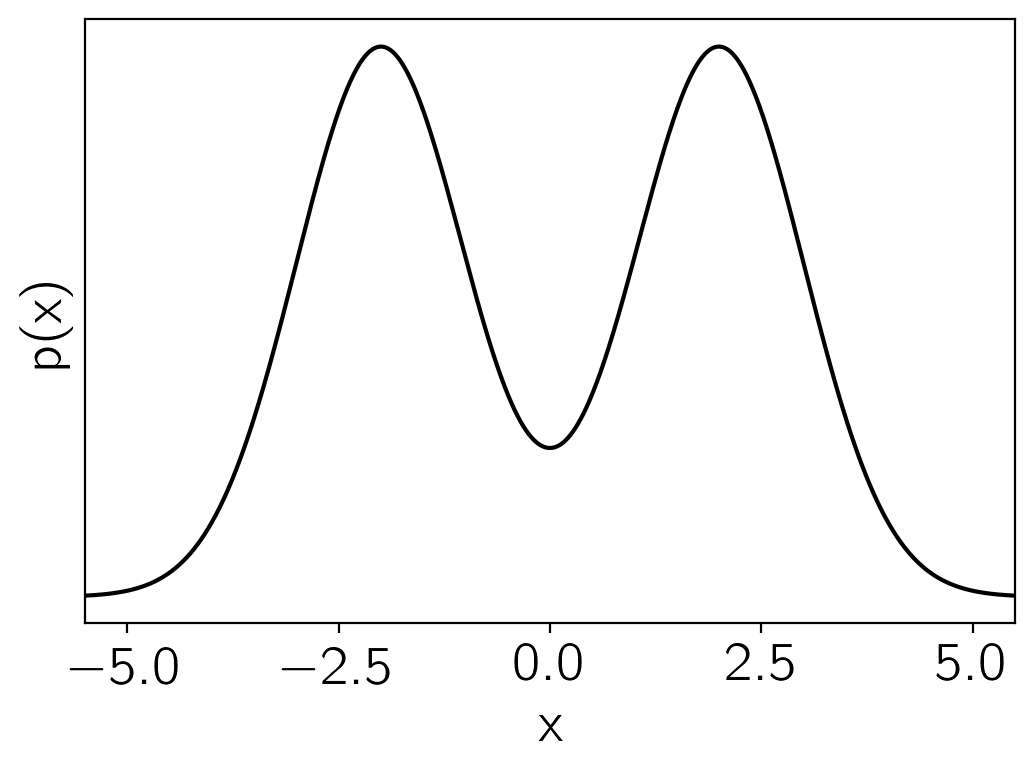
One of the most important new features included in the version 3 release of emcee is the interface for using different “moves” (see Moves for the API docs). To demonstrate this interface, we’ll set up a slightly contrived example where we’re sampling from a mixture of two Gaussians in 1D:
import numpy as np
import matplotlib.pyplot as plt


def logprob(x):
    return np.sum(
        np.logaddexp(-0.5 * (x - 2) ** 2, -0.5 * (x + 2) ** 2,)
        - 0.5 * np.log(2 * np.pi)
        - np.log(2)
    )


x = np.linspace(-5.5, 5.5, 5000)
plt.plot(x, np.exp(list(map(logprob, x))), "k")
plt.yticks([])
plt.xlim(-5.5, 5.5)
plt.ylabel("p(x)")
plt.xlabel("x");
Now we can sample this using emcee and the default
moves.StretchMove:
import emcee
np.random.seed(589403)
init = np.random.randn(32, 1)
nwalkers, ndim = init.shape
sampler0 = emcee.EnsembleSampler(nwalkers, ndim, logprob)
sampler0.run_mcmc(init, 5000)
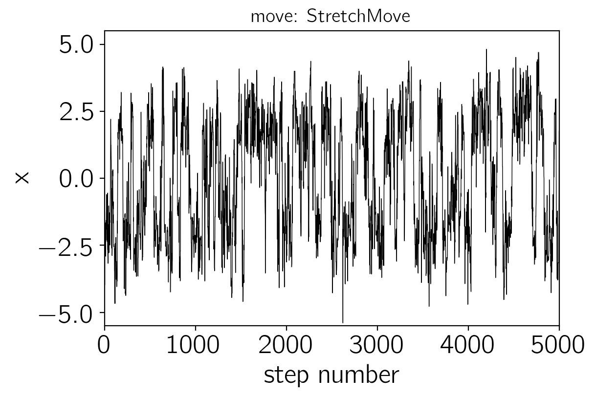
print("Autocorrelation time: {0:.2f} steps".format(sampler0.get_autocorr_time()[0]))
Autocorrelation time: 40.03 steps
This autocorrelation time seems long for a 1D problem! We can also see this effect qualitatively by looking at the trace for one of the walkers:
plt.plot(sampler0.get_chain()[:, 0, 0], "k", lw=0.5)
plt.xlim(0, 5000)
plt.ylim(-5.5, 5.5)
plt.title("move: StretchMove", fontsize=14)
plt.xlabel("step number")
plt.ylabel("x");
For “lightly” multimodal problems like these, some combination of the
moves.DEMove and moves.DESnookerMove can often
perform better than the default. In this case, let’s use a weighted
mixture of the two moves. In deatil, this means that, at each step,
we’ll randomly select either a moves.DEMove (with 80%
probability) or a moves.DESnookerMove (with 20% probability).
np.random.seed(93284)

sampler = emcee.EnsembleSampler(
    nwalkers,
    ndim,
    logprob,
    moves=[(emcee.moves.DEMove(), 0.8), (emcee.moves.DESnookerMove(), 0.2),],
)
sampler.run_mcmc(init, 5000)

print("Autocorrelation time: {0:.2f} steps".format(sampler.get_autocorr_time()[0]))

plt.plot(sampler.get_chain()[:, 0, 0], "k", lw=0.5)
plt.xlim(0, 5000)
plt.ylim(-5.5, 5.5)
plt.title("move: [(DEMove, 0.8), (DESnookerMove, 0.2)]", fontsize=14)
plt.xlabel("step number")
plt.ylabel("x");
Autocorrelation time: 6.49 steps
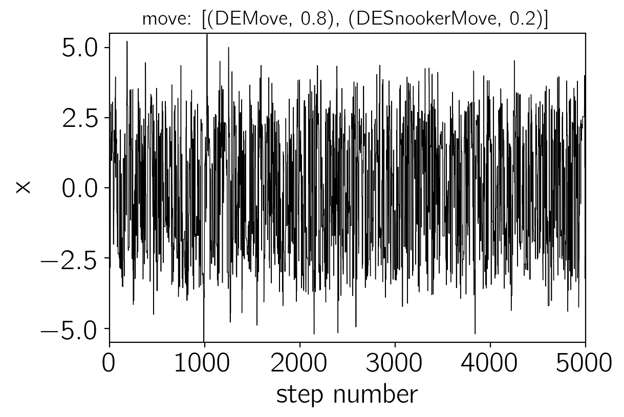
That looks a lot better!
The idea with the Moves interface is that it should be easy for users to try out several different moves to find the combination that works best for their problem so you should head over to Moves to see all the details!